Do the valuation of assets under the QE/QT parameters set by the central bank in response to recessions, asset valuation collapses, and countervailing consumer inflation, self assemble into defined time-based fractal patterns?

The argument for this proposition is contained under an identifiable US 1807 36/90/90/54 year ongoing umbrella quantitative x/2.5x/2.5x/1.5-1.6 fractal pattern with valuation lows in 1842/43 after the valuation asset high Panic of 1837, with the 90 year low in 1932 after the valuation high in 1929, and with the 1932 to 2021 90 year high valuation in (November) 2021.

The asset-debt valuation system’s two quantitative self-assembly patterns are composed of either one: a four phase pattern: x/2-2.5x/2-2.5x/1.5-1.6x which represents the big picture 1807 36/90/90/54-56 year US hegemony pattern or two: a x/2-2.5x/1.5x-2.5x three phase pattern. The nomenclature in identying the subunits of the 4 phase pattern are arbitrarily named as the first, second, third, and fourth fractal of the fractal series and for the three phase phase pattern, the first, second, and third fractal. Hence the 4 phase fractal is composed of 4 fractals (subfractals) and the three phase fractal is composed of 3 fractals(subfractals). With the central bank’s QT response to consumer inflation, the length of the second fractal of each series determines the ideal length of the first base fractal and hence the ideal length of the third (and fourth) fractal.

Since 1932, the third 90 year and fourth 54-56 year fractals are composed of two interpolated fractal patterns which also conform to the two patterns defined above. The first is a 10-11/20-21/20-21 year fractal series :: x/2x/2x ending in 1981-82 and the second series a 13/31-33/31-33/20 year pattern ending in about 2074. The 1981-1982 13 year base fractal is composed of a 3/7/5 year fractal series followed by two subseries: the first a 3/7/7 year fractal series ending in 2009 and a second 4/10/6-7 year fractal series ending in 2025 or 2026. The second yearly fractal series is composed of a series of interpolated monthly fractal series: the sequential monthly fractal series since 2009 have been 5/12/10/7; 3/8/6; 8/17/17; 10/26/16; and 7/17/14 of 17 ending in May 2023. A super-bubble second fractal nonlinear devaluation is expected in the 13/31-33 year time frame, whose second fractal nonlinearity is described in the 2005 web site opening page,

Since the March 2020 low valuation, the weekly fractal series is 33/72/49 of 60-61 weeks. With the historical QT to contain consumer inflation, the ideal base of the second 72 week second fractal was shortened to 29 weeks, which became the determinant base time period for the third decay fractal. The third decay fractal for the March 2020 three phase series started on 14 March 2022 and is composed of a 10/23/18 of 18/12-13 week series ending in May 2023. A global hard landing crash economic recession will generate another monthly fractal series ending in 2025 to 2026.

Using the the Russell 2000, from 14 March 2022, the 60-61 week third fractal is composed of 42+/107/84 of 84-86/63 days :: x/2.5x/2x/1.5x.

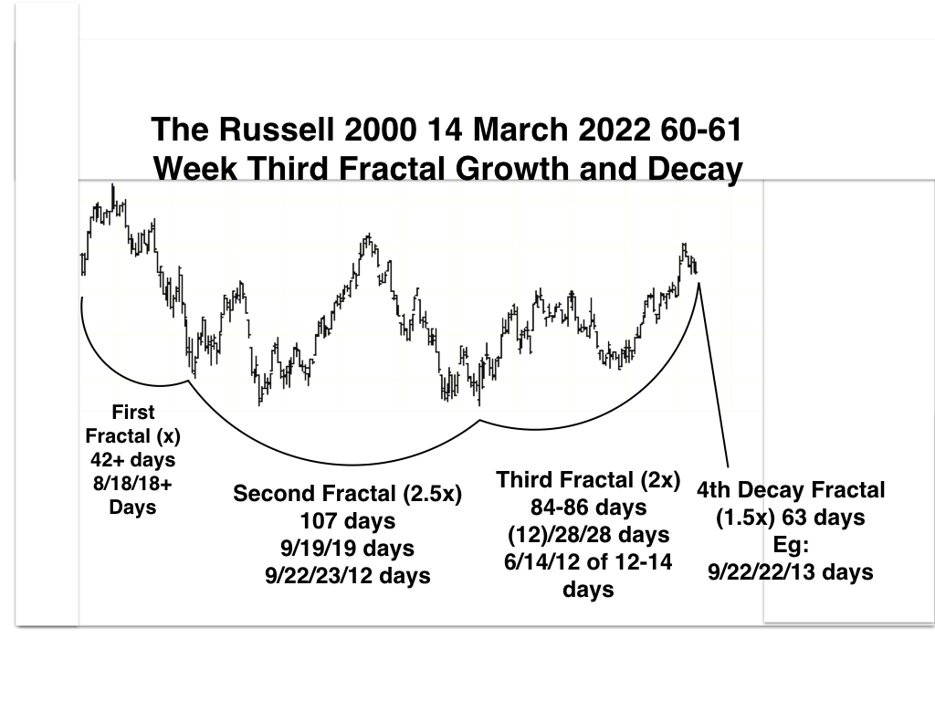
Over the next 63 trading days and ending in May 2023 expected a nonlinear crash in the 2009 US asset Super Bubble created by the US central bank through extraordinary QE and ex nihilo money creation activity.

The US Asset-Debt system is undergoing an 1807 36/90/90/54 year  :: x/2.5x/2.5×1.5-6x Self-Assembly Great Fractal Cycle with asset valuation lows in 1842/43 and 1932, and a high in 2021.

The 90 year Third Fractal and the 54 year Fourth Fractal are composed of two interpolated equity fractal series  starting in 1932. The first series was a 10-11/21/21 year fractal ending with a yearly low in 1981/82. The second equity series, the Volcker US bond low series, began in 1981/82: and consists of 13/33/33/18-20 years, ending in 2074-76

The Volcker Second Fractal series started with a 3/7/5 year 13 year base  equity fractal from 1981/82 to 1993/94.   The second fractal to this first base was compose of two sub-series:  3/7/7 year series ending in 2009 and a 4/10/4 of 6-7 year series ending in 2025-2026.

Volcker’s 30 year bond prices decreased from their 15.1% high  in 1981 to 0.8 percent in 2020.  The lowering of bond rates correlated to both one: rapid money supply expansion with the accumulation of 93 trillion dollars of total US debt rising to an unprecedented 350% of GDP,  and two: with an asset  super bubble. Composite US equity valuations rose to the November 2021 90 year  Third Fractal high and housing valuation prices rose beyond the 2007 peak price to wage earning ratio. Financial  corporations, enabled by low mortgage  interest rates and advantaged availability to capital, drove valuations up, crowding out wage earners.

The Fed’s recent mini Volcker attack on consumer price inflation has taken  the fed funds rate in less than a year from 0.25  to 4.25-4.50, an unprecedented 1800% increase above the nadir rate. This percentage increase has never happened before. With the massive  US debt to GDP ratio and extreme housing valuations, this accelerated interest rate increase will result in a nonlinear 13/30-33 year 1981-82 second fractal  asset valuation price collapse.

At 93 trillion dollars of debt supported by only 26 trillion GDP,  mostly service job related, the US asset-debt system cannot tolerate 3.5-4.7 interest rates. During the US Fourth Fractal’s next 52-54 years, interest rates will not only return to zero levels, they will (must), like Germany, become negative for  to the asset debt system to survive. The disparity between the working class and those individuals and entities with disproportional access to capital and having financial assets grown disproportionally by negative rates, will become greater. The rich will enable a sympathetic populist to gain control of the political system.

The final 6-7 years of the 2009 4/10/6-7 year second subfractal series is likely composed of two subfractals : a March 2020 8/17/13 of 13 of 17 month subfractal series with a possible repeat of a similar monthly fractal sequence.

Over the next 11-12 trading days expect nonlinear declines in the Wilshire, Gold, and Bitcoin to conclude the Equity March 2020 8/17/13 of 17 month subfractal series.

The US 1807 36/90/90/54 year asset debt valuation cycle.

Cycles  of debt expansion occur causing increases in asset valuations until bad debt cannot be sustained, then  bad debt liquidation and asset valuation declination synergistically feed on each other. 

1932 ended the US Second Fractal 90 year debt expansion and collapse cycle and November 2021 ended its Third Fractal apogee 90 year finale debt expansion and asset peak valuation cycle.  

A 1932  first subfractal 10-11/21/21 year debt expansion cycle ended in 1982 with  Volcker’s interest rate hike solution to contain consumer  price inflation.

The initial cycle of the 1982 Second Subfractal, secondary to the 1932 to 1982 51 year First Subfractal cycle, was composed of a 13 year 3/7/5 year cycle ending in 1994.  The second subcycle to this 13 year base is compose of a series of sub fractals: a 1994 16 year 3/7/8 year cycle ending in 2009 and thereafter 2 subseries; 2/4/5 years and 2/4/4 years. Each cycle unit has ended with an underlying trend line containing all of the preceding valuation lows as bad debt was liquidated.

If the asset debt system maintains its previous consistency,  a valuation nonlinear low for the SPX will be about 1000, a 75 % nonlinear decrease from the current valuation.  From 2009 the two cycles are each roughly 17/35/35  months.

Expect a riveting hard landing for asset owners as asset valuations fall to long term trend lines.