The construct of a Global Macroeconomic System operating and self-assembling  in a time based  mathematical fractal progression of maximum asset valuation and debt growth and, thereafter at peak valuation, necessary and deterministic  asset devaluation and  debt default, which the elegantly simple Lammert quantitative fractal system provides,  represents  a useful tool for characterizing and understanding  the complex integrative system.

Topics:

• 4 February 2020 : The average MSCI World Equity Index valuation  high,  MSCI in monthly, weekly, and daily fractals  from the beginning of the final1982 second subfractal series  2009 third fractal
• The 1932 US Hegemonic Great Third Fractal  Final peak bubble
• A comparison of the  terminal 1921 and 2009 respective third fractal portions of the 90 Year Great US  Hegemonic 1843 Second Fractal and 1932 Third Fractal Fractal

4 February 2020 : The average world equity Index valuation high (MSCI)current MSCI Lammert daily fractal series from its 2 October 2019 average daily low was  16/40/32 days ::  x/2.5x/2x. The 32nd day of third fractal 4 February 2020 represents the current average peak high valuation for the index.

For MSCI, the world equity index, 4 and 5 February 2020 were the all time average and absolute peak valuation days of this index.

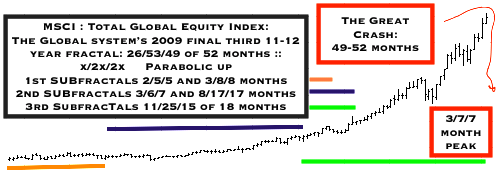
The monthly terminal fractal series from the adjusted nonQE supported and  non troubled assets federal acquisition time frame in September 2009 is 26(orange)/53(purple)/49(green) months  :: x/2x/2x.  The third 49 month third  subfractal is composed of 11/25/15 months with the 15 month third subfractal of this final 2009 subfractal series composed of  3/7/7 months :: x/2-2.5x/2-2.5x

 

The 3/7/7 months terminal third fractal represent a weekly fractal pattern since the December 2018 low of  11/23/(9)/19 weeks where (9) is a shared interpolated fractal between the second and third subfractal  for a current third of a third of a third of 1932  US hegemonic 90 year third  fractal series of 11/28/22 weeks : x/2.5x/2x. The terminal 22 weeks represents the third fractal subseries of this 11/28/22 weeks subfractal series.

By the simple saturation fractal math of the asset debt macroeconomic system, 4 and 5 Februrary 2020 appear to be peak saturation days for the  global system.

The 1932 US Hegemonic Great Third Fractal  Final Peak Bubble:

The final equity bubble of the 1932 US Hegemonic Great  Third Fractal was created during the time period of 2008-2020 with a combination of illiquid trouble assets federal acquisition,  Central Bank Quantitative Easing, Sovereign Money Printing, and Corporate Tax Slashing resulting in corporate buybacks of their own stocks.   Part of the debt explosion  has trickled down to the base population, who have then  leveraged mostly newly created  service  jobs to incur citizen debt for student loans, automobiles and credit card purchases.

Very telling is that only 1.5 million US  jobs have been added since 2000 averaging 75,000 a year with about 30 million boomers retiring since 2010.  The system is a Ponzi scheme with the poignant exception that developed countries have the power to print money and honor their 90 year old social contracts with their working and tax paying citizens.

A visit to US Federal Debt clock provides perspective. 

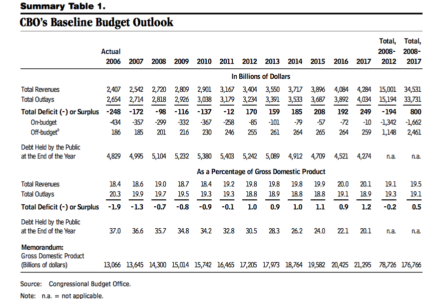
The CBO does not factor in its calculations  expected fractal nonlinearities, bad debt liquidation,  asset devaluation and expected recessions.  A review of the 2006 CBO budget outlook (below) shows the disparity between projected deficits and ones that occurred with the collapse of the housing bubble.  The 2008-2020 propelled bubble will be worse than this is the expected degree of nonlinear asset devaluation occurs.

The Great 1932 US Hegemonic Third 89 year Fractal series: is elegantly simple.

The US 90 year third fractal dating from the low in 1932 is composed of two  subfractal series

1. From the 1932 low ending on 12 August 1982 :  51 years 
2. And from the August 1982 low to present : 39 years

From 1932 to 1982:  a x/2x/2x fractal series defined by valuation lows : 10-11/21-22/21-22 years is easily observable. 

From the  August 1982 low: 9/20/12 years 

1982-1990  :  9 years

1990-2009. : 20 years

2009-2020  : 11+ years

 The 4 and 5 February  peak valuation days  for the MSCI global index fell in the third 19 week fractal of a 24 December 2018 low 12/30/19 week :: x/2.5x/1.5-1.6x  fractal series.  A final 1.6x Fibonacci proportionality growth peak with a 12 week base lies in the  terminal portion of a 18/36/90/89 year series and  is a reasonable maximal growth terminus. This 11/20/19 week fractal series represents  the  terminal third portion of  a 11 February 2016 low  three phase subfractal series  which is the third terminal portion  for the 6 March2009  low which began the terminal major third fractal subseries and  ended a  20 year second subfractal dating from 1990 to 2009 with  a 9 year  fractal  base starting from  the August 12  1982 valuation low and ending 1990.  12 August 1982 again  concluded a 51 year 1932 to 1982 first  fractal subseries of 10-11/21-22/21-22 years. 12 August 1982 began the second yearly  subfractal series of 9/20/12 years of the 90 year third fractal of a 36/90/89 year series beginning in 1807 with a 18 year initiating fractal starting in about 1790. 

The third of the third of the third of the … Lammert growth fractal

1932 : begins the US hegemonic  Great Third Fractal  (First US Great Fractal 1807 to 1842-43: 36 years; Second  US Great Fractal 1843-1932)

1982: ends of first 51 year subfractal series starting in  1932: 10-11/21-22/21-22 years)and begins the  second 39-40 year subfractal series.

1982 -1990 … first fractal of the second and final  subseries : 9 years

1990-2009 … second fractal:  20 years

2009 to present … third fractal series:  11 years

A comparison of the  terminal 1921 and 2009 respective third fractal portions of the 90 Year Great US  Hegemonic 1843 Second and 1932 Third Fractals

The  11 + year terminal portion of the 1843 US Hegemonic Second Fractal as compared to the 11 + year terminal portion of the 1932  89 year US hegemonic Third Fractal.

1919–1921: Bear market. The Dow lost 46.6% of its value in just over 21 months, before reaching a low of 63.90 on August 24, 1921.

What was the stock market increase from 1921 to peak 1929?

Between 1921 and 1929 the stock market grew by 600% with the Dow Jones Industrial Average rising from 63 points to 381 points.  This rapid growth was based on cosumer credit to purchase newly manufactured items and the practice of ten percent margin purchase of equities.

Great Depression’s  DJIA  maximum devaluation  occurred on July 8, 1932; 32 months after its 1929 peak.   On this day in 1932, the Dow Jones Industrial Average fell to its lowest point during the Great Depression, closing at 41.22. From its highest level in 1929, the Dow had a devaluation of nearly 90 percent.

The sharp stock market decline in the wake of the 1929 crash not only affected Wall Street. It also undermined consumer consumption as foreign trade, industrial production and employment fell precipitously for the ensuing decade. In political terms, it led to the 1932 victory of Franklin D. Roosevelt, the first Democrat to be elected president since 1916.

Aug 24 1921 to 8 July 1932         11 years  – 2/12 months

6 Mar 2009 to  current 7 Feb 2020    11 years – 1 month 

6 March 2009:  On this day, the Dow Jones Industrial Average hit its lowest point of the financial crisis of 2008 and 2009.  The S&P 500 was trading at 683.38 and the Dow dipped as low as 6,469.95.

 

In March 2009, it seemed as if nothing could stop the plummeting stock market as U.S. investors feared the entire banking industry was on the brink of collapse. The largest U.S. banks had been bailed out by the government via the Troubled Assets Relief Program, and investors struggled to understand just how bad the situation was.

The current SPX high: 29,286.92.   From  its 2009  683 low, this represents a 450% rise. 

The construct of the Macroeconomic System operating and self assembling  in a time based  mathematical fractal progression of maximum asset valuation and debt growth and, thereafter at peak valuation, necessary and deterministic  asset devaluation and  debt default which the Lammert quantitative system provides  represents  a useful tool for characterizing and understanding  the system.

 

 

 

 

The Quantitative History of American Macroeconomics: The Greatest Ever Asset-Debt Macroeconomic Quantitative Collapse ::  The Terminal 51/113/103 Day :: x/2-2.5x/2x Growth Fractal

Nonlinear Asset Valuation Collapse… 

Starting near the time of the endorsement of the US  constitution, it is the current and contemporary  time  frame of January 2020, that  is the historical time frame of the quantitative  asset  peak valuation  and the terminal portion of the 90 year Third Great Fractal cycle of the Great US Hegemonic Fractal Growth Cycle –  ending in a  classic  maximally extended x/2.5x/2.5x of x/2.5x/2.5x/1.5x  :: 36/90/90/54 year pattern.

Since its inception, US (and prior hegemonic and global) periodic  job growth is synergistically associated with  large expansions of credit and debt-based growth on that job expansion which causes further job expansion causing further credit expansion until a saturation area of asset production and relative overvaluation is reached.

It is the observational theory of this web site that this known qualitative cyclical process is a time dependent (dt) and easily recognizable quantitative process.

The system’s assets’s valuations turn negative when the acceleration dt/dt of debt expansion of the base population  slows to zero. The system then undergoes nonlinear asset valuation  collapse and devaluation as bad debt undergoes default and debt based assets are ‘revalued’ and repossessed at a lower valuation and placed on an oversupplied market relative to reduced jobs and nonlinearly contracted available credit.

Starting about 1790 and ending in 1807-08 , an 18 year ‘initiating  US fractal’ for a hegemonic three phase fractal cycle of debt dependent asset growth and terminal collapse was completed. 

This 18 year (1/2x) initiating fractal cycle generated a x/2.5x/2.5x cycle of 36/90 and currently 89 years with respective cycle ends in 1842-43, 1932 and a projected end in 2020-2021 for a 36/90/89-90 year  three phase fractal cycle.

The final cycle after 2020-21 is expected to be about 54 years. This will be a revealing and educational  cycle globally as it will become evident that current debt  and future  social debt obligations cannot be mathematically paid for by future inflationary  economic expansion by its base population as it has been in the past 235 years of  growth cycles.  The only  forced option is sovereign money printing to pay for the accumulated debt and  past social contract  promises. This option has as its 2008  precedent in  HR 1424.

Since the 1932 global  Great 2nd fractal low,  there have been two easily recognizable  three phase fractal series:

1. a 50 year three phase cycle  of 10+/21/21 years  :: x/2x/2x  ending in 1982 and
2. and 39 year three phase cycle of  9/20/11 of 11-12 years  expected to nadir in 2020 to 2021.

The 89-90 year Great US Third Fractal’s short 2009 terminal third fractal series of 11-12 years matches the ending of 12 year third fractal from 1921 to 1932 which ended the 1842-43 to 1932 90 year Great Second US Fractal. 

The 2009 three phase fractal series is a 31/53/currently 48 month cycle

The third final 48 month  fractal current  is a 11/26/currently 14 month sequence.

The 14 month sequence is composed of 51/113/currently 103 days or x/2-2.5x/2x growth sequence. Collapse is imminent.

Expect a well defined  self organized decay fractal over the 14 trading days of historical devaluation possibly a 4/8/6 day devolution.

The fractal pattern of summation commodity valuations, i.e., CRB is well aligned with that the US equities.  Just as the CRB index collapsed in parallel with global equity valuations in 2008-2009, expect a similar sharp decay pattern but over the next 14 trading days.

 

From the December 2018 low

7/18/18/10 of 11 weeks

From the 1 June 2018 low : 18/45/45/28 {(2)5/12/ 9 of 12)} days