This time is different.
Nonlinearity for the asset debt macroeconomic system is a sudden daily, weekly, monthly, yearly mathematical fractal collapse of asset prices and zombie enterprises whose valuation growth and sustainability are based on prior easy credit, expansion of the money supply, and resulting gross overvaluation.
With the US’s winning of WW2(without destruction of its infrastructure), its resulting position as the global reserve currency, and its renewed uncoupling to a gold standard on 15 August 1971 (the Nixon shock), the US has been able to cascadingly expand its money supply via money printing and debt creation with a series of (fractal) asset price collapses with nadirs in Sept-Oct 1974, 19 October 1987, July and October 2002, March 2009, 6 May 2010 and March 2020.
The M1 money supply.
The US money supply in 1929 was 26.5 billion and decreased to 19 billion in 1932, a drop of 28%.
From 1929(26.5B), the money supply increased to 226.5 billion in August 1971, an increase of 855% and an average increase of 20 % per year over the 42 year interim. After the Nixon Shock of decoupling from the gold standard in 1971, the US money supply increased from 226.5 billion to 3.97 trillion in Feb 2020, a 1766% increase over 49 years or an average of 36% per year.
The ‘Trump Shock’ and Covid occurred in 2020 with an increase in the US Money supply from February 2020 at 3.98 trillion to February 2021 to 18.36 trillion, a 463% increase in the money supply in single year (as compared to the prior average annual increase of 20 % and 36% in years before and after the Nixon Shock.)
The primary cause of US inflation was this one year 463 % increase in the US money supply sustained by the 2023 8-9 % COLA increase in social security payments for the 64 million + retired and disabled US citizens.)
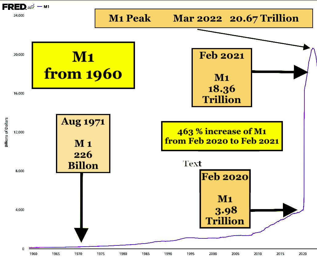
M1 Money supply peaked at 20.7 trillion in March 2022 and has since decreased via QT and higher interest rates to about 18.4 trillion, a ten percent decrease over 15 months and beginning to rival the monthly average decrease % rate of the 1929 to 1932 M1 collapse. With a coming nonlinearity in asset prices, the decrease in money supply could exceed that of the decline during the 1929 to 1932 nadir.
The Federal reserve has predicted that post pandemic reserve savings for US citizens starting at 2.1 trillion in 2021(23 months ago) will reach zero by October 2023. https://www.youtube.com/watch?v=MQSgLJfsepA
What macroeconomically to the asset-debt system will happen after such extraordinary central bank QE/QT policies?
The current mathematical monthly decay fractal model for the Bank of Shanghai is a November 2017 9/20/18 month x/2-2x/2x 3 phase decline followed by a July 2021 3 phase decay decline of 9/19 of 20/12-18 months :: x/2-2.5x/1.5-2x.
For the Wilshire the asset valuation growth (QE) and (QT) decay model is a 4 phase March 2020 8/18-20/18-16/12- 13 month decay fractal series.
Fractal groupings are determined by trend lines connecting the lowest valuation of day one of the fractal series to the lowest valuation of the last day of the fractal series.
For the composite Wilshire a base fractal (subfractal 1) of 52 days is observable from the low on 13 Aug 2023 to 24 May.
Subfractal 2 is potentially composed of a x/2-2.5x/ 1.5x’ a three phase decay series; x’ = 2-2.5x divided by 2.5.
x is observable as 30 days from 24 May to 10 July.
2-2.5x is potentially 63 days, a 10/21/20/15 day series ending 5 Oct 2023.
Subfractal 3 (1.5x’) is potentially a 37-38 day series. 63 divided by 2.5 equals 25 days times 1.5 equals 37-38 days ending 27/28 November.
27/28 November could represent a double bottom
and serve as the base fractal for a 38/80/48 day :: x/2-2.5 x/1.5x’ series and completing a March 2020 33/72-73/72-73/44-45 week :: x/2-2.5x/2.5x’/1.5x’ 4 phase series.
The peak decay fractal series from 31 July starts on 27 July and consists of subfractal one: 3/7/6/4 days, or 17 day, a base for a 3 phase decay fractal series.
(Note the downward trend line connecting the lows of 27 July and 18 Aug with all intervening days above the trend line.
Subfractal 2 appears to be a 34 day 6/11 of 15/15 day (three phase) fractal (decay series)ending 5 October.
Subfractal 3 of 37-38 days ending 27-28 November would complete a 13 August 52/128-129 day :: x/2.5x subfractal one and subfractal two series.
From 27 July 2023 the 3 phase decay series would be 17/34/37 days :: x/2x/2-2.5x.
An advantageous characteristic about fractal mathematical models is that a working model can be quickly determined to be wrong. The above model is consistent with empirically derived and observable simple laws of time-based fractal asset valuation growth and decay http://www.economicfractalist.com/blog/ (see 31 August posting) which appear to quantitatively govern asset growth and decay valuation pathways – qualitatively created more and more since late 2008 by historically extreme central bank cyclical QE/QT policies.